Quantization and the Need for TPUs

Original post published here. More about the author here.
Machine learning can be compared to a play you see in a theatre. Imagine you are the producer of this play and that the director has assured you that he has rehearsed the play at least 10 times. Now all you can do is hope that all the actors play their part well, while you are seated in the audience praying that nothing goes awry backstage!
Now imagine the backstage as consisting of rows and rows of TPUs (tensor processing units) and your actors are the weights on your neural network. We are just going to rely on the fact that all that happens backstage including the makeup, coordination, and prepping of the scenes run smoothly. But what really happens behind the curtains is pure magic.
Or is it?
When you are talking about training a particular neural network, that is the top-level abstraction, what really goes on during prediction underneath, is pure quantization. In my previous blog, I mentioned how signals are pre-processed, but another interesting terminology related to that is quantization.
What really is quantization?
When you are dealing with a large amount of data, one has to keep in mind the ever-changing values that one might obtain. Especially, signal data with large SNR (Signal to Noise Ratio) in them, which causes different sets of data to be produced. The best way to deal with such signal data is to apply truncation or rounding off such values, typically making it a many-to-few mapping.
Why do we need to quantize?
To understand why quantization arose, imagine you have 100 different tasks to be performed backstage, but the theatre given to you is really tiny. How will you manage?
The answer is by optimizing the tasks. Divide tasks between individuals in such a way that you require less time and space.
But how do you manage that with a neural network? For that we need to dive into the history of neural networks and why the need for such optimization techniques arose, helping us understand the reason behind the present structure of TPUs.
Neural networks, as we all know, mirror the actual neural nerves running through our bodies. The use of neural networks was split into two ways, primarily for the brain and then for AI. In the late 1940s, Hebbian learning or unsupervised learning paved the path for the usage of neural networks in artificial intelligence. But unsupervised learning could be easily be performed on calculators.
With the use of the theory of backpropagation in 1975, the need for a larger neural network arose, as more complex calculations could no longer be handled by calculators. This neural network was able to modify the weights across the network. But there were fewer machines to tackle such a huge computational power.
On the other end of technology, the world was rapidly moving towards its first 8-bit microprocessor in 1971. After many failed attempts with the Intel 8080, Intel was finally able to produce its first ever 8008 8-bit microprocessor.
It is very important for us to understand the basic 8-bit calculations because as suggested before, it was necessary to optimize and thereby map every computation performed by a neural network up to the basic level.
How do you exactly map a 32/24 bit neural network layer to an 8-bit chip?
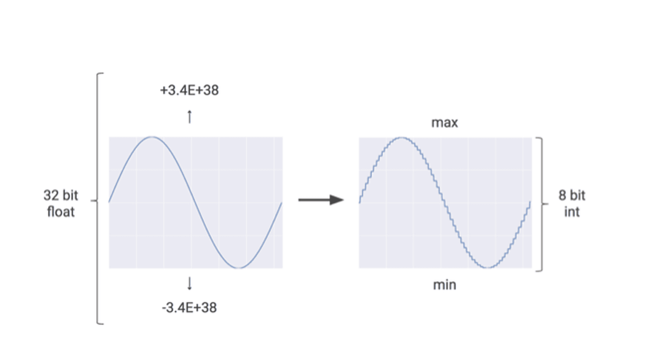
To know about the mapping process, let us look at a popular section presented by TensorFlow:
Neural network training is done on 32-bit floating-point integers. 32-bits are used because during training, the changes given by backpropagation to the weights are usually quite small; so small that they become apparent only on 32-bits.
However, this creates a problem during inference or while running the neural network. 32-bit multiplication takes a lot of time and a lot of computational power to evaluate. Even though the accuracy is high, in most cases, it becomes too complex a calculation.
The solution to this was to convert the 32-bit values into 8-bit values, so as to reduce the computational cost. Although this leads to a slight loss in accuracy, in edge computing and real-time applications, the gain in speed is far more desirable than the loss of accuracy.
TensorFlow has recently released an API that converts 32-bit floating-point integers into 8-bit integers.
Generally, all weight values in the neural network are in a small range. Say, for example, from -8.342343353543f to 23.35442342554f. In TensorFlow, while doing quantization, the least value is equated to 0 and the maximum value to 255. All the values in between are scaled inside the 0 to 255 range.
In these examples, notice that if we take even negative values of a floating scale, it is easier to convert it to a range of 0 to 255 scale.
But what really happens inside a neural network?
The integer values are the basics of the neural network computation, but when we take an entire layer, each network performs its own set of predictions, which are further quantized.
Consider a basic ReLU operation performed by your neural network. This is usually done in 32-bit, but our aim is to map it down to 8-bits. Consider the second image – we use the minimum and maximum functions in order to convert the input float to 8-bit value and then feed it to the QuantizeRelu to remove any unnecessary or redundant float values.
Understanding “Fake Quantization Operators”
Although quantization seems to be an easy enough task to do, in reality, there are a lot of things that you have to take into account to get it to work. The quantization that TensorFlow provides currently is called “Fake Quantization”. The reason for this is something called the True Zero problem.
When we quantize one range of numbers into another range, the numbers often lose their precision. For example, a number like 2.3443789539f in 32-bit might get represented as a 4 in 8-bit. The problem arises when we try to convert it back to its 32-bit value in which case it might get converted to 2.3457938493f, which is a drift of about +0.001.
This is not a problem as the loss of precision is throughout all the values and neural networks are generally good at dealing with such noise. However, the problem arises when we are dealing with zero values.
Zero values are used more often than you might think in machine learning. For example, they are used while padding images for input into CNN’s; they might also be used to initialize certain values and even ReLU outputs that are zero.
It is important that the zero value does not drift, as it might cause a problem later on. TensorFlow currently does not support a fix for the True Zero problem; hence, the quantization operation given by them is called fake quantization.
But is quantization really the solution to all our memory, space, and optimization problems?
According to Google Cloud Platform, quantization can be compared to the rain outside your window. Their argument is that you only need to know how heavily or lightly is it raining. Similarly, in case of neural networks, you only need to know the approximate accuracy, which can easily be given in an 8-bit integer value.
Their argument will hold in most cases, but there are some scenarios where quantization does not play out fairly.
Why not choose quantization?
Quantization can be a boon or a bane to the world of machine learning. On one hand, because of quantization, doing calculations on IoT devices in real-time and on the edge can become very easy. This is because the low precision can make calculations simpler, faster, and less computationally expensive.
In fact, this is why TensorFlow included implementation of quantization in their API in the first place – to put less load on their TPUs (more on this later) and to reduce the time taken to perform calculations.
However, in other cases, quantization can be a bane. Although, there have been very few studies on the relationship between quantization and its effect on accuracy, when notes, the effects are quite drastic. Quantizing a neural network can reduce the accuracy by a large percentage. While this might not be as serious a problem in edge computing applications, the effects could be quite serious in some other places.
Take self-driving cars, for example, where a difference of a few percentages could make the difference between a safe drive and a crash. So while quantization is powerful, as it can make computing a lot faster, its applications should be considered carefully.
So how is quantization tackled? Let us now look into edge computing and its application. Quantization was vastly popular even before the rise of the Tensor Processing Unit, especially with edge computing.
Quantization and Edge Computing
Traditional Internet of Things (IoT) infrastructures have two main parts – the edge and the cloud. The edge is the part of the system that is closest to the source of data. It includes sensors, sensing infrastructures, machines, and the object being sensed. The edge actively works to sense, store, and send that data to the cloud.
The cloud, on the other hand, is a huge centralized infrastructure where all the data is stored and analyzed. This part of the system resides far away from the source of the data. Traditionally, data would be collected and sent to the cloud for analytics, the results from the analytics would then be sent to the edge, where a user would read the analysis or a machine would perform certain actions. However, this leads to latency in the system and a huge chunk of the IoT system’s run-time would be spent in sending data back and forth between the cloud and edge.
In edge computing, data is not sent to the cloud for analysis, instead, the analysis is done right there in the edge. This can be useful in cases where internet connectivity is not available, like mines, and in cases where fast computing is necessary, like in autonomous vehicles.
However, the problem with this approach is that most of the analytics work is computationally very expensive and the edge systems (which are usually simple microcontrollers) cannot handle these calculations.
In this case, quantization can be a boon. Changing the computation from 32-bit to 8-bit floating point numerical has been shown to reduce computational tasks, at times, by up to 30% without a significant reduction in accuracy.
The Rise of TPUs
Everything that we have discussed in this article was at the heart of building the Tensor Processing Unit in 2015 when it was first used at Google’s data centers. After the official release of the Tensor Processing Unit in 2016 at Google I/O, TPUs have been used for various purposes including Google Street View, text processing, and Google Photos for saving over a million photographs by a single TPU.
The picture still seems incomplete, doesn’t it? I have just talked about a single-player backstage – this just a peek into the magic behind the curtains. But what does the entire set really look like? Stay tuned for our next blog on architecture on TPUs to see more of the theatre set.