Applications of Signal Processing in Machine Learning

Original post published here. More about the author here.
Data is available abundantly in today’s world. However, it is noisy most of the time. In this article, Archana Iyer discusses some filter processing techniques that can help us get a better quality of data.
With the advent of IoT, many types of medical data are now available in the form of sensor data. This data can be from wearable devices, like Fitbit, or from implanted medical devices. But like all sensor data, this data is prone to noise and misleading values.
Machine Learning, along with IoT, has enabled us to make sense of the data, either by eliminating noise directly from the dataset or by reducing the effect of noise while analyzing data.
What is Pre-processing?
In a world of 7 billion people, data is rich and abundant. This has helped several data scientists all across the world to perform various studies on such data. However, every data wrangler has come across data which is very noisy in nature. It is difficult to make sense of the data from that perspective. Hence, to feed a proper set of data into a model, data pre-processing is performed.
There are several pre-processing techniques that exist including box-plots, ignoring missing values and sometimes even manually processing the data.
This isn’t the first time we have had to deal with noisy data though. Processing noisy signals has been a huge concern over the last few decades. Signal processing techniques developed today are very robust and effective models. In this article, we will port some processing techniques from the audio and signal field and use them to process sensor data. We will take a look at a few filter processing techniques that can help us.
Filters in Audio Processing
Audio filters are a lot different than filters in CNNs. Filters in CNNs perform convolution operations, whereas in audio processing, filters are used to stop or filter out certain signals.
Some of the common ones used to remove noisy data from a signal are explained in this section.
Low Pass Filters: Devices often record high values due to random spikes in current or voltage. Often times, the device might be put through some adverse conditions, like high G-Forces, temperatures or pressure. During these times the chances of recording very high values increases.
Low pass filters can help eliminate the high value data, as it allows only the low values to pass through and ‘stops’ high values from going through the filter.
The limit for a low pass filter can be set manually or they can also be learnt by using machine learning. This is a simple, but powerful, technique that can remove anomalous data.
High Pass Filters: A high pass filter is the opposite of a low pass filter. Instead of allowing low values to pass through, it allows high values to pass through. This can be used to eliminate zero values during training.
Band-pass Filter: Band-pass filters combines the best of both worlds. It prevents both high and low values from passing through. As the name band-pass implies, it allows a band of values to pass through the filter.
Kalman Filters: Kalman filters that are used specifically to remove noise from data. The Kalman filters were most prominently used in spacecrafts to track the location of the spacecraft and the moon.
Traditional tracking algorithms use a sort of integrating controller that has a way of summing up errors in measurements. This leads to large drifts from the actual output in the long run. The Kalman filters were able to change that.
The Kalman filter works in two steps – predict and update. In the first step, the value of the output is given along with a degree of uncertainty. In the update state, the output of the filter is updated based on the new inputs and the current and previous uncertainties. This is a recursive algorithm that gives increasingly accurate outputs with each step, which makes them more powerful.
Why Did the World Start Paying Attention to Signal Processing?
Digital Signal Processing like many other fields of science traces itself to a very unruly period in history. Interestingly, most of the developments can trace their origins to either World Wars or National Security requirements.
In the 1960s, when the Soviets started building nuclear weapons, the Americans got interested as well and set up sensors all around Russia. Unfortunately, like every hardware, the sensor data was full of noise and could not be analyzed. The Fourier Transform was then adapted for practical use to properly pre-process data for analysis.
I’ll try to explain to you how Fourier Transforms work and how we process signals to fit our needs.
Fourier Transforms
During J. F. Kennedy’s presidency, IBM was working on this interesting project of understanding Fourier Transform. Unfortunately, they did not have the proper resources, and it took them almost six months to implement their theories.
Today, we have it much easier. FFT or Fast Fourier Transform can be implemented using a few lines of python code:
from scipy.fftpack import fft
import numpy as np
audio = np.random.rand(N, 1) * 2 - 1
audio_fft=fft(audio)
Now we’ll try to understand this processing in a simpler way.
Fast Fourier Transform (FFT): The advent of Digital Signal Processing started with the understanding of how computation takes places in the real world. Let’s take a scenario of Argand plane geometry, which is popularly used in the complex planes:

In a divide and conquer scenario, let us take a number and try to divide it in all possible manners. We can think of multiple scenarios where we can use either two 8s or four 4s to reach the number 16.
From this plane, we can say that in order to comprehend the nth roots of unity, we just need to split the multiplication to half, and then decompose correspondingly, thereby reducing our complexity from O(n2) to O(nlogn).
Now, let us take a simple sinusoidal wave on python and perform the necessary FFT on it.

An important thing to remember is that FFT can be applied to only certain frequencies. Hence, we have taken a normal sine wave to show noise data in order to understand how it works.
import numpy as np
import matplotlib.pyplot as plt
from scipy.fftpack import fft, ifft
from scipy.signal import hamming
N = 1024
T=1/512
x = np.linspace(0.0, N*T, N)
sinewave = np.sin(50.0 * 2.0*np.pi*x)
sinefft=fft(sinewave)
xfft=np.linspace(0.0, (N*T), N)
plt.plot(xfft, sinefft)
plt.show()

Windowing
Windowing, as the name suggests, is used to take a small window of the dataset to apply a particular processing to it, as a way to make a signal finite rather than periodic in nature.
Applying windows in the time domain also causes ripples in the frequency domain. Windows are applied as another pre-processing technique before the application of DFT or FFT. There are different kinds of windows available in the scipy.signal package.
The following code illustrates the use of a Hanning window:
import numpy as np
import matplotlib.pyplot as plt
from scipy.fftpack import fft, ifft
from scipy.signal import hanning
N = 1024
T=1/512
x = np.linspace(0.0, N*T, N)
sinewave = np.sin(50.0 * 2.0*np.pi*x)
sinefft=fft(sinewave)
xfft=np.linspace(0.0, (N*T), N)
hng=hanning(N)
win=fft(sinewave*hng)
plt.plot(xfft, win)
plt.show()
The output of the above code looks like this:

Discrete Fourier Transform (DFT): As the name suggests, a Discrete Fourier transform is a sinusoidal signal to be decomposed into various frequencies, allowing it to be “discrete” in nature.
But how does the DFT work in practical sense? Let us look at the equation of a typical DFT:

This equation only gives a superficial representation of how each discrete signal might be split within the frequency range. Understanding this at a deeper level lets us look into how a DFT might affect a complex piano version of a song “The Blue Danube.”

The image here shows how the sample music looks on a spectrogram. As we apply DFT to it, we can see the clear change in the signal.
The following code is used to perform a spectrogram on the music:
def createA(N,input_length,hop):
FH=np.dot(createF(N),hanWindow(N))
A=np.zeros(((2*input_length-1)*N,input_length*N),dtype=complex)
for i in range(2*input_length-1):
A[i*N:(i+1)*N,i*hop:i*hop+N]=FH
plot(A)
def plot(matrix):
matrix_abs=np.abs(matrix)
plt.figure()
plt.imshow(matrix_abs)
plt.xlabel("Column")
plt.ylabel("Row")
plt.colorbar()
This spectrogram showcases lower frequency decomposition giving a discrete sample for the entire song.

What Type of Dataset Should We Target?
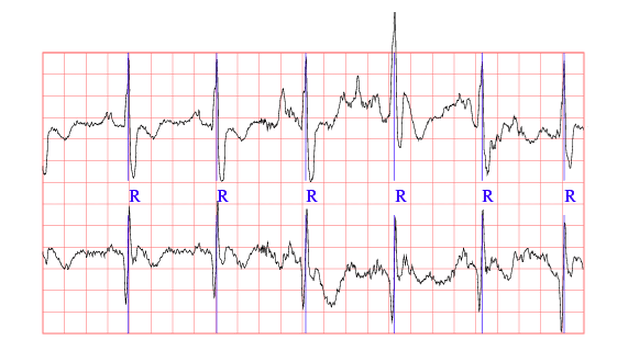
Let us take a very simple dataset of ECG recordings of the MIT BIH Noise Stress Database, which has a 12-hour ECG recording and a 3-hour noise recording.
There was a signal to noise ratio during the noisy segments which are recorded as below:
| Record | SNR (dB) | Record | SNR (dB) |
| 118e18 | 18 | 119e18 | 18 |
| 118e12 | 12 | 119e12 | 12 |
| 118e06 | 6 | 119e06 | 6 |
| 118e00 | 0 | 119e00 | 0 |
| 118e_6 | -6 | 119e_6 | -6 |

This is one of the various examples where several signal processing methods can be applied.
Removing noise from a very dirty data set through pre-processing is one of the first steps to applying filters and implementing such data to the real world scenarios.
Conclusion
One of the various fields where audio processing can be applied is medical data, which can help millions of lives all around the world. This process can take healthcare to another level by presenting a data goldmine to the scientists.
The very first attempt of its kind was by an IBM group that used previous recorded blood samples to determine if there were any traces of cancer in it.
Today, the process has evolved a lot. Google DeepMind is working with cancerous tissues to understand how radiation can be further improved. This type of cutting edge application in healthcare is exactly the right place to start using signal processing in ML.